Optimization of work distribution using one-dimensional bin packing algorithm_2.Algorithm (1)
2. One-dimensional Bin Packing Algorithm
2.1. One-dimensional Bin Packing Algorithm Type
The four representative algorithms of Bin Packing are as follows.
- Next Fit: Fill in last bin or new bin
- First Fit: always seek and fill from the first bin
- Worst Fit: Find and fill the bin that can fill the current item with the largest remaining size among all bins
- Best Fit: Find and fill the bin that can fill the current item with the smallest remaining size among all bins.
In addition, a much more optimized result can be obtained by sorting all items in descending order of size and applying each algorithm. Considering the method of applying descending sort, it can be said that there are a total of 8 algorithms.
The following inputs and constraints are used for explanation. (The name of the item in the input is omitted and only the size is described)
- Input: 26 57 18 8 45 16 22 29 5 11 8 27 54 13 17 21 63 14 16 45 6 32 57 24 18 27 54 35 12 43 36 72 14 28 3 11 46 27 42 59 26 41 15 41 68
- Constraint: 80 (max size of one bin)
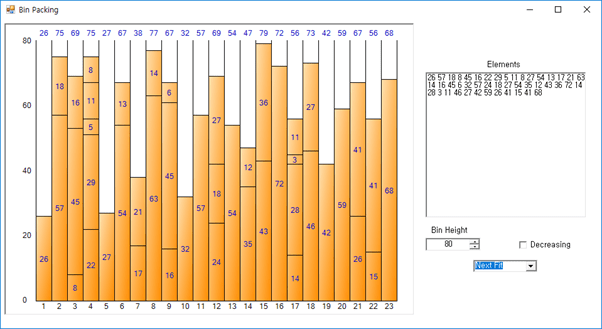
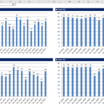
Note: This case data and constraints are http://www.developerfusion.com/article/5540/bin-packing/ The basic data of the Bin Packing Sample Application that can be downloaded from . The screen of this sample application is as follows.
Let's take a detailed look at the pseudo code, processing process, and execution result of each algorithm.
2.2. Next Fit Algorithm
For each item, the last bin is filled if it can be filled, and if it cannot be filled, a new bin is created and filled. Next Fit is the simplest, but the result is not optimal.
// Pseudo code
item(1)을 새로운 Bin(1)에 채운다.
for (i=2; i<=item 개수; i++) {
    j = 마지막 Bin index
    if (item(i).Size <= Bin(j).남은공간Size) {
        Bin(j)에 item(i)를 채운다;
    }
    else {
        새로운 Bin(j+1)을 생성하고 item(i)를 채운다;
    }
}
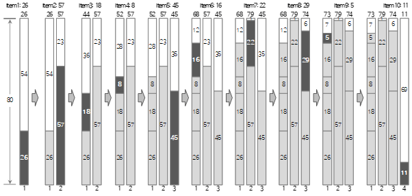
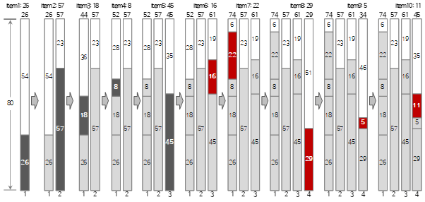
Let's take a look at the process up to the <10>th among the above input values in the figure below.

The first input value <26> creates a new Bin1 and fills it.

The second input value <57> is larger than the remaining size (54) of bin (1) and cannot be filled, so a new bin (2) is created and filled.

Since the third input value <18> is smaller than the remaining size (23) of the current bin (2), it is filled in bin (2).
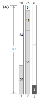
The fourth input value <8> is larger than the remaining size (5) of the current bin (2) and cannot be filled, so a new bin (3) is created and filled. As you can see here, the Next Fit method does not use even if there is space left in the bin that has already passed. Accordingly, a lot of wasted space may occur.

Since the fifth input value <45> is smaller than the remaining size (72) of the current bin (3), it is filled in bin (3).
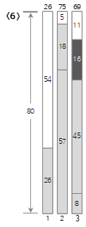
Since the sixth input value <16> is smaller than the remaining size (27) of the current bin (3), it is filled in bin (3).
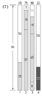
The seventh input value <22> is larger than the remaining size (11) of bin (3) and cannot be filled, so a new bin (4) is created and filled.
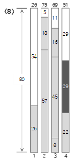
Since the eighth input value <29> is smaller than the remaining size (58) of the current bin (4), it is filled in bin (4).
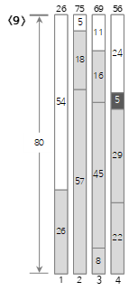
Since the ninth input value <5> is smaller than the remaining size (29) of the current bin (4), it is filled in bin (4).
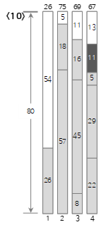
Since the tenth input value <11> is smaller than the remaining size (24) of the current bin (4), it is filled in bin (4).
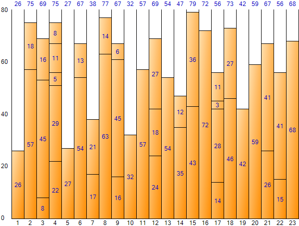
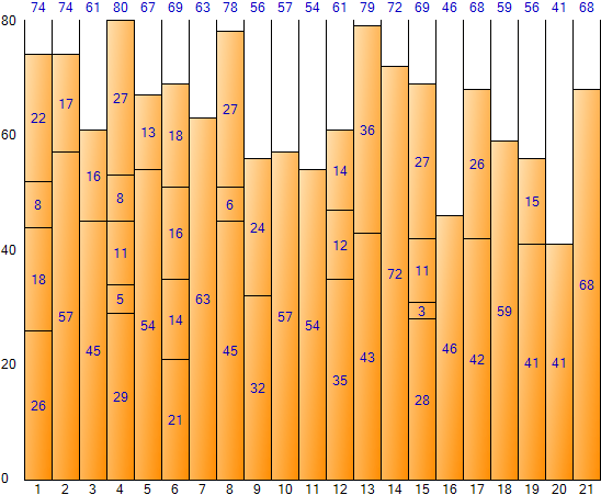
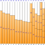
If you keep filling up to the last item in the Next Fit method, you can get the following result. (Result screen of Bin Packing Sample Application)
As can be seen in the figure above, the result of the Next Fit method is difficult to see as the optimal result because of the large waste of space. However, it has the advantage of fast execution speed due to the small number of iterations. The total space is 1,840 (size 80 per bin * number of bins 23), and the total remaining space is 488, and the space inefficiency is about 26.52% (488/1,840).
2.3. First Fit Algorithm
For each item, check whether the entire bin can be filled, fill it in the first bin that can be filled, and if not, create a new bin and fill it.
// Pseudo code
item(1)을 새로운 Bin(1)에 채운다.
for (i=2; i<=item 개수; i++) {
    for (j=1; j<=Bin갯수: j++) { // 항상 처음 Bin부터
        if (item(i).Size <= Bin(j).남은공간Size) {
            // item(i)를 채울 수 있는 Bin(j) 탐색
            Bin(j)에 item(i)를 채운다;
            exit for;
        }
    }
    if (마지막 Bin까지 탐색해도 채울 수 없었으면) {
        새로운 Bin(j+1)을 생성하고 item(i)를 채운다;
    }
}
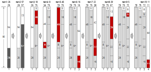
The process of filling up to the first 10 of the above input data with the First Fit method is shown in the figure below.
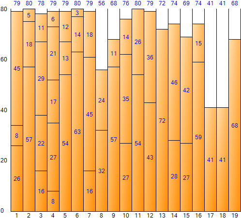
Filling the entire input data in this way gives the following result: (Result screen of Bin Packing Sample Application)
First Fit method has the advantage of less space wastage than Next Fit and smaller total space due to fewer bins. However, the disadvantage is that the execution time is long due to the relatively large number of iterations. The total space is 1,520 (size 80 per bin * number of bins 19), and the total remaining space is 168, and the space inefficiency is about 11.05% (168/1,520).
2.4. Worst Fit Algorithm
For each item, fill the bin that can be filled with the largest remaining size among all bins, and if there is no suitable bin, a new bin is created and filled.
// Pseudo code
item(1)을 새로운 Bin(1)에 채운다;
for (i=2; i<=item갯수; i++) {
    long lMaxRemainSize = 0;
    long lMaxRemainSizeBinIndex = 0;
    for (j=1; j<=Bin갯수: j++) {
        // 남은공간Size가 가장 큰 Bin 탐색
        if (lMaxRemainSize < Bin(j).남은공간Size) {
            lMaxRemainSize = Bin(j).남은공간Size;
            lMaxRemainSizeBinIndex = j;
        }
    }
    if (item(i).Size <= Bin(lMaxRemainSizeBinIndex) {
        // 남은공간Size가 가장 큰 Bin에 item(i)를 채울 수 있는 경우
        Bin(lMaxRemainSizeBinIndex)에 item(i)을 채운다;
    }
    else {
        새로운 Bin(j+1)을 생성하고 item(i)을 채운다;
    }
}
The process of filling up to the first 10 of the above input data by the Worst Fit method is shown in the figure below.
In the figure, the red item indicates a case where the filling method is different from the first fit method.
Filling the entire input data in this way gives the following result: (Result screen of Bin Packing Sample Application)
Worst Fit method wastes less space than Next Fit, but wastes more space than First Fit. The total space is 1,680 (size 80 per bin * number of bins 21), and the total remaining space is 328, and the space inefficiency is about 19.52% (328/1,680).
2.5. Best Fit Algorithm
For each item, it is a method of finding and filling a bin that has the smallest remaining size among all bins and can fill the corresponding item, and if there is no suitable bin, a new bin is created and filled.
// Pseudo code
for (i=2; i<=item갯수; i++) {
    long lMinRemainSize = 제약조건으로 입력한 Bin의 최대 크기;
    long lMinRemainSizeBinIndex = 0;
    for (j=1; j<=Bin갯수: j++) {
        // 남은공간Size가 가장 적으면서 item(i).Size를 채울 수 있는 Bin 탐색
        if (oBin(j).남은공간Size >= item(i).SIze) and
           (lMinRemainSize > oBin(j).남은공간Size)
            lMinRemainSize = Bin(j).남은공간Size;
            lMinRemainSizeBinIndex = j;
        }
    }
    if (적합한 Bin을 찾았으면) {
        Bin(lMinRemainSizeBinIndex)에 item(i)을 채운다;
    }
    else {
        새로운 Bin(j+1)을 생성하고 item(i)을 채운다;
    }
}
The process of filling up to the first 10 of the above input data in the Best Fit method is shown in the figure below.
In the figure, the red item indicates a case where the filling method is different from the first fit method. Comparing the process with First Fit and Worst Fit gives a clear understanding of the method.
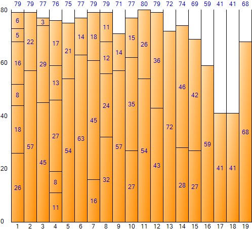
Filling the entire input data in this way gives the following result: (Result screen of Bin Packing Sample Application)
The best-fit method generally achieves the most optimal results, but has a disadvantage in that it takes a long time to execute due to the large number of iterations. The total space is 1,520 (size 80 per bin * number of bins 19), and the total remaining space is 168, and the space inefficiency is about 11.05% (168/1,520).
The result of the First Fit and Best Fit methods having the same number of bins and the same residual space is unique to the input data used as an example and may not always be the same.
We have looked at each algorithm so far, and next we will compare the method of applying descending sort and the application result of each algorithm.
<< List of related articles >>
- Optimization of work distribution using one-dimensional bin packing algorithm_1.Overview
- Optimization of work distribution using one-dimensional bin packing algorithm_2.Algorithm (1)
- Optimization of work distribution using one-dimensional bin packing algorithm_2.Algorithm(2)
- Optimization of work distribution using one-dimensional bin packing algorithm_3.Implementation (1)
- Optimization of work distribution using one-dimensional bin packing algorithm_3.Implementation (2)
- Optimization of work distribution using one-dimensional bin packing algorithm_4.Attachment
- One-dimensional Bin Packing Tool Recent Changes (as of March 21, 2021)
- Work distribution optimization tool using one-dimensional bin packing algorithm Full Contents, Download
